Portfolio
Poisson Data Clustering
Project Description
In this project I try to extend the data clustering algorithm presented in a paper by Casagrande et al. titled "Hamiltonian-Based Clustering: Algorithms for Static and Dynamic Clustering in Data Mining and Image Processing" to a more general setting. Hamiltonian dynamics live in an even dimensional space, and my aim is to instead work on a more general space that allows the Hamiltonian dynamics to live on an odd dimensional space. The primary assumption is that the data live in the phase space and at each data point a Gaussian function is assigned to it. Hamiltonian systems tend to evolve along trajectories in the phase space where the Hamiltonian remains constant and when the motion is period that corresponds to closed loops in the phase space. The idea to employ Hamiltonian systems to find the boundaries of the sets.
As it is with Hamiltonian dynamics, it requires the points to be defined on a cotangent bundle, and cotangent bundles are symplectic manifolds. The limitations of that are that symplectic manifolds are even dimensional manifolds and thus for the data clustering algorithm to work, it requires the data to be even dimensional. The main example used in aforementioned paper obtain data in the form of images, which is a two-dimensional plane. The complications arise when the data are gathered from the real world, say data that lives on the surface of a sphere. In this case the data lives in a three-dimensional space and it cannot be a symplectic manifold. One possible solution, suggested in the paper [1], is to embed odd-dimensional data into an even-dimensional space. At this stage, we try to circumvent such solution by not adding an extra dimension.
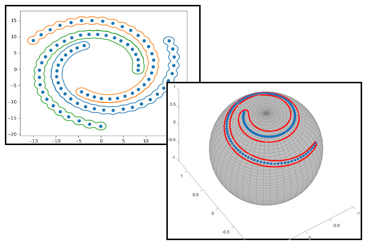
We consider an example in three dimensions where we have \(N\) data points, \(\mathbf{x_k} \in \mathbb{R}^3\) for\(k=1, \dots, N \), for a spiral on the surface of a sphere. The aim is to find a set, \(\mathcal{C}\), whose elements \(\mathbf{x_i}\) satisfy certain condition, and in this case the condition is that the elements of the sets needs to be adjacent to each other.
This figure shows the result of Poisson data clustering algorithm. The data point are represented by solid blue dots and the boundary of the set is represented by the red curve.
References:
[1] - D. Casagrande, M. Sassano and A. Astolfi, "Hamiltonian-Based Clustering: Algorithms for Static and Dynamic Clustering in Data Mining and Image Processing," in IEEE Control Systems Magazine, vol. 32, no. 4, pp. 74-91, Aug. 2012.
Deep Learning and Fluids
Project Description
In this exploratory project, the link between deep learning and fluid dynamics is investigated. A detailed exposition for this project can be found on my personal project page. This enables us to find the limit of deep learning system when both the number of neurons and the number of layers approaches infinity.Further, results of this project are being written in two seperate academic papers: the first focuses on the application Hamilton-Jacobi theory to deep learning and the second regards multisymplectic geometry formulation of deep learning.
Currently, there has been an interest in representing deep learning problems in terms of dynamical systems as was discussed in "A Proposal on Machine Learning via Dynamical Systems" by E. In fact, dynamical systems appear in many neural network architectures, such as recurrent neural network, echo state machines, and spiking neurons to name a few. For the case of spiking neurons, the continuum limit yields a hyperbolic partial differential equation and the field of study is known as neural field theory. This point of view allows for training neural networks to be cast as an optimal control problem. This is of great interest as it provides links between deep learning, hydrodynamics, symplectic and multisymplectic geometry as it is being explored in the papers in preparation. The hydrodynamics connection can be viewed as an extrapolation of the work of Bloch et al in "An Optimal Control Formulation For Inviscid Incompressible Ideal Fluid Flow" .
References:
[1] - W. E. "A proposal on machine learning via dynamical systems." in Communications in Mathematics and Statistics 5.1 (2017): 1-11.
[2] - A. M. Bloch, D. D. Holm, P. E. Crouch and J. E. Marsden, "An optimal control formulation for inviscid incompressible ideal fluid flow," Proceedings of the 39th IEEE Conference on Decision and Control (Cat. No.00CH37187), Sydney, NSW, 2000, pp. 1273-1278 vol.2.
Forecasting
Project Description
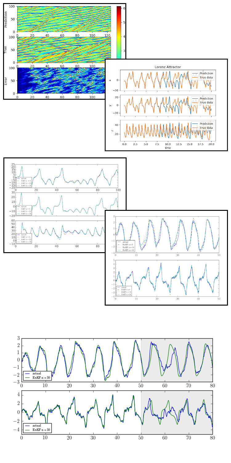
During my undergraduate studies I took courses on signals and systems and Bayesian inference. I became interested in studying systems and using mathematical models to not only control them, but also predicting their behaviour. There are a number of ways, depending on the type of system and available data; one can forecast the states of the system in the future. I mainly worked on three methods, and they are: reservoir computers, ensemble Kalman filter and symbolic regression.
One of the types of neural network that intrigued me the most is reservoir computers, which are a variant of recurrent neural networks. What makes them interesting is that their efficiency in training, where they don't suffer most of the pathologies and complexities of recurrent nerual networks. Employing them to forecast chaotic systems were presented in many papers such as Pathak et al's "Using machine learning to replicate chaotic attractors and calculate Lyapunov exponents from data." This captured my attention as I wanted to use such networks to implement data-driven control scheme of a black-box system. In the process of learning and implementing reservoir computers, I published a blog post on Medium.com, which can be accessed here.
The second method used for forecasting is the Ensemble Kalman filter. Unlike the previous method, filtering does not substitute the model it enhances the current model. Such algorithms are used in many applications, from implementing feedback controllers to data assimilation and forecasting. This project is my implementation of Ensemble Kalman filter. The filter is an algorithm that, given a set of measures, generates the optimal estimate of the desired quantities through a recursive processing. The Ensemble Kalman filter and it uses Monte Carlo methods to approximate the statistics of the system. The algorithm relies on having the knowledge of the system and its measurement dynamics. In addition to that, the statistical description of the noise associated with the system, the measurement error and the uncertainty of the used dynamic models.
To showcase my implementation of ensemble Kalman filter to estimate the state of the van der Pol oscillator, a nonlinear dynamical system, described by
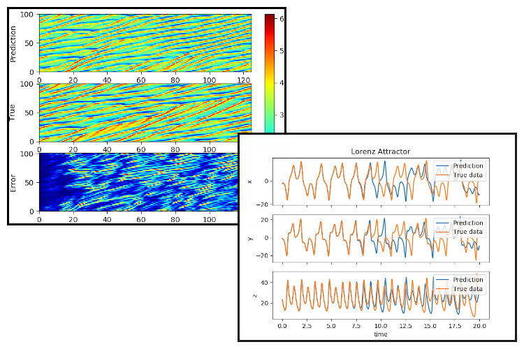
$$ \begin{bmatrix} x_0^{k+1} \\ x_1^{k+1} \end{bmatrix} = \begin{bmatrix} x_0^{k} + \Delta t \, x_1^{k} + w_0\\ x_1^{k} + \Delta t \, \left( \mu \left(1 - (x_0^{k})^2 \right)x_1^{k} - x_0^{k} \right) + w_1 \end{bmatrix} $$ where \(\Delta t\) is the time step, and here it was chosen to be \(0.01\), \(\mu = 1\), and \(\bar{w} \sim \mathcal{N}(0, Q)\) is a normally distributed random number with covariance \(Q = \mathrm{diag}(0.0262, 0.008)\). Another example used to test the implementation of the ensemble Kalman filter is the Lorenz 63 model, whose solution produces the famous Lorenz attractor. The dynamics of the system are described by
$$ \begin{bmatrix} x_0^{k+1} \\ x_1^{k+1} \\ x_2^{k+1} \end{bmatrix} = \begin{bmatrix} x_0^{k} + \Delta t \, a \, \left(x_1^{k} - x_0^{k} \right) + w_0\\ x_1^{k} + \Delta t \, \left( x_0^{k} \left( b - x_2^{k}\right) - x_1^{k} \right) + w_1 \\ x_2^{k} + \Delta t \, \left( x_0^{k} \, x_1^{k} - c x_2^{k} \right) + w_2 \end{bmatrix} $$ and the measurement is done according to $$ \bar{y}^{k+1} = C \bar{x}^{k+1} + \bar{v} $$With \(\bar{w} \sim \mathcal{N}(0, Q)\), where \(Q = \mathrm{diag}(0.01, 0.03,0.1)\) and \(\bar{v} \sim \mathcal{N}(0, R)\), where \(R = 0.003\). The figures show the approximated state using the measured data \(y\).
The third method for forecasting is symbolic regression. The aim is instead of finding a network's weights, or changing the model's parameters, symbolic regression finds a mathematical expression that closely fits the observed data. Evolutionary programming is often used to find the mathematical expression. I have used symbolic regression, however not for forecasting but for the autonomous navigation project.
References:
[1] - J. Pathak, Z. Lu, B. R. Hunt, M. Girvan, & E. Ott, "Using machine learning to replicate chaotic attractors and calculate Lyapunov exponents from data" in Chaos: An Interdisciplinary Journal of Nonlinear Science, 27(12), 121102. (2017).
Reinforcement Learning
Project Description
While learning about stochastic optimal control, I came across reinforcement learning which is a machine learning paradigm that is frequently used when the mathematical model is unavailable. However, that was before the introduction of deep Q-networks and things have changed drastically thereafter. Here are few projects that I worked on to help me learn about reinforcement learning:
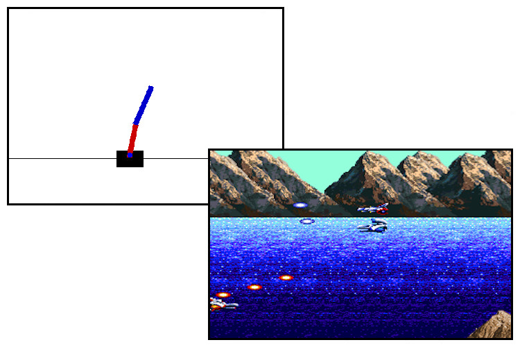
Stabilising an inverted double:
One of the entry problems in reinforcement learning is stabilising an inverted pendulum on a moving cart. The controls are either move the cart left or right depending on where the pendulum is starting to swing. Here a similar problem is considered and instead of a single pendulum a double pendulum remains stationary on a moving cart. This renders the problem more challenging as the double pendulum is a chaotic system, but despite that it possesses two equilibrium point. At this point, a deep Q-network is used to stabilise the inverted pendulum by moving the cart either left or right.
Playing a side scrolling shoot 'em up:
Deep Q-network came to prominence when it was used to learn and play Atari games. Here instead of using the standard Atari games, a slightly different game is considered, which is coded from scratch. The game is based on Thunder Force IV. In order to use reinforcement learning to teach a computer to learn video games, either use a convolutional neural network to "read" the screen, or access an emulator's memory directly. The third option is to code a game from scratch and use it as a control system and feed the states directly to DQN. For this reason the game was coded using Gym AI.
AI & ML Driven Autonomous Navigation
Project Description
A few years ago I was part of Queen's Mostly Autonomous Sailboat Team, and my role was to program a boat to sail autonomously. At that time I wanted to implement artificial intelligence controller for the navigation, but due to hardware constraints, the idea was abandoned. Things have changed, hardware-wise, since last time I worked on such problems and now with the advances in artificial intelligence it is the right time to revisit it again. This project focuses on using data driven approach to programming robots to navigate environments and follow a prescribed trajectory.
The trajectory tracking problem is a well-known problem in control theory, where the goal is to find an input to the dynamical system that would result in a path close the predefined one. However, it requires an exact mathematical model for the vehicle or boat and instead of deriving a model beforehand, the response of the controlled system to predefined commands is observed. Then a regression method is applied to find the mathematical model. The result can be seen in the figure on the right.
Another way of tackling navigation problem is implementing an evolutionary robotic paradigm. Here the vehicle is Reed-Shepp type car where the speed and steering are the controls. The vehicle is equipped with five forward facing proximity sensors whose readings are fed, along with the vehicle's position, as inputs to the control neural network. The control here is implemented using feed-forward multilayer perceptron. Other network architectures can be used and it is on the todo list to use reservoir computers for control. The most evolutionary process is implemented using genetic algorithms, here particle swarm optimisation is used to evolve the weights of the control neural network. My C++ implementation can be found here
Another control theory problem I am interested in is the using geometric integrators for controlling non-linear mechanical systems, for example, attitude control for satellites. One of such integrators is the Clebsch integrator, where the position of the satellite is rotated using a SO(3) Lie group action. The optimal control that connects two orientations belongs to a specific space known as coadjoint orbit. We can use the properties of motion on the coadjoint orbit to simplify the optimal contol problem. The figure of the right shows a cube where the vertex $(1,1,1)$ is rotated so that it is positioned at $(1,1,-1)$
Pseudospectral Optimal Control
Project Description
This project remains an ongoing work to implement pseudospectral control methods, presented in a paper by Fahroo and Ross titled "Legendre Pseudospectral Approximations of Optimal Control Problems", using Python. The idea of the said method is to use pseudospectral approximations of functions to solve optimal control problems. An optimal control problem has three core components: cost function, state-constraint and dynamical constraint. Implementing an efficient numerical scheme for one component does not guarantee that it would approximate the other two well. Psuedospectral methods address such issue by guaranteeing that the approximation works for all three components.
This project's repository can be found hereReferences:
[1] - M. Ross, and F. Fahroo. "Legendre pseudospectral approximations of optimal control problems." in New trends in nonlinear dynamics and control and their applications. Springer, Berlin, Heidelberg, 2003. 327-342.
Restricted Boltzmann Machine
Project Description
One of the types of neural networks that caught my attention was Restricted Boltzmann Machine. I came across RBMs after reading David MacKay's book "Information Theory, Inference, and Learning Algorithms" [1]. A Restricted Boltzmann Machine is a class of Markov random field, which is an undirected graph used to visualise probability distributions. I worked on this project mainly to learn about Restricted Boltzmann Machines and Deep Belief Networks by understanding how they work by implementing them. RBMs is used in a number of real-world applications such as classification and collaborative filtering. The main source used to learn about RBMs is a paper by Fischer and Igel titled "An Introduction to Restricted Boltzmann Machines" [2]. The code is intended to be used for future research project related to the field of information geometry.
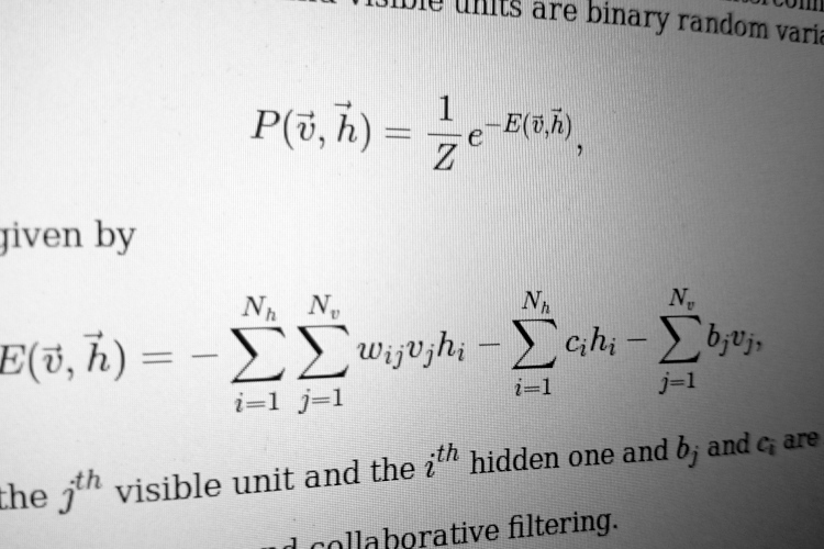
An RBM consists of \(N_v \) visible units \( \vec{v} \), which represents observed data and \( N_h \) hidden units \(\vec{h} \). The units are interconnected, however, units from the same type are not connected with each other. The most common used type of RBMs, the hidden and visible units are binary random variables, that obey a Binomial distribution. The probability distributions over the model is given by
\( P(\vec{v}, \vec{h}) = \frac{1}{Z}e^{-E(\vec{v}, \vec{h})}, \)
where \(Z \) is the normalising factor and \( E(\vec{v}, \vec{h})\) is the energy given by\( E(\vec{v}, \vec{h}) = -\sum_{i=1}^{N_h}\sum_{j=1}^{N_v} w_{ij}v_jh_i - \sum_{i=1}^{N_h}c_ih_i - \sum_{j=1}^{N_v}b_j v_j, \)
where \(w_ij \) is the weight assigned to the connection between the \(j^{th} \) visible unit and the \(i^{th} \) hidden one and \(b_j\) and \(c_i \) are biases. The repository for my implementation of RBM can be found here.References:
[1] - D. J.C. MacKay. "Information theory, inference and learning algorithms". Cambridge university press, 2003.
[2] - A. Fischer, and C. Igel, "An introduction to restricted Boltzmann machines. In Iberoamerican Congress on Pattern Recognition." (2012, September), (pp. 14-36). Springer, Berlin, Heidelberg.
Geometric Numerical Integrator Library
Project Description
This is an ongoing project whose aim to provide an STL C++ library for geometric integrators (variational, generating functions, variational multisymplectic). The full library is not available for the general public, however a small snippets of the library, in form of simple examples, are uploaded on Github and here are two examples:
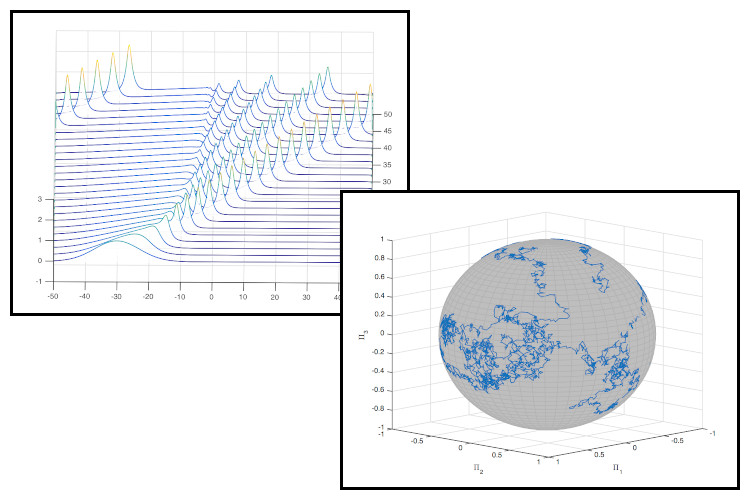
Stochastic Rigid Body
Here we solve the Euler-Poincaré equation for the rigid body whose dynamics, in terms of angular momentum, are given by
\( d\Pi = \Omega \times \Pi \, dt + \sum_k \Xi_k \times \Pi \circ dW_k^t \)
where \(\Omega \) is the angular velocity and it's relation to the angular momentum is \( \Pi = \mathbb{I} \Omega \). Normal numerical schemes struggle solving this type of equations, and for that reason geometric integrators are used. The figure shows that the numerical solution stays on the sphere at all time.Camassa-Holm Equation
Another interesting equation that I worked on is the Camassa-Holm equation given by:
\( u_t + 2\kappa u_x - \alpha^2 u_{xxt} + 3 u u_x = \alpha^2 2 u_x u_{xx} + \alpha^2 u u_{xxx} \)
This is an example of a partial differential equation with a Hamiltonian structure and an infinite number of conserved quantities. Solving it numerically is challenging and to preserve the geometric structure of the equation, geometric integrators are used and they are implemented using my geometric integrators library.
Navier-Stokes Equation
Along with Hamiltonian systems, the library can be used to solve the celebrated Navier-Stokes equation for incompressible fluid, which in the vorticity form is given by
\( \partial_t \omega + u\cdot \nabla \omega - \nu \Delta \omega = 0 \)
where \( \omega = \mathrm{curl} u \) is the vorticity and \( u \) is the velocity vector field. A lid-driven cavity benchmark problem was used to test the code and the result of the vorticity is shown in the second figure. The code can be found here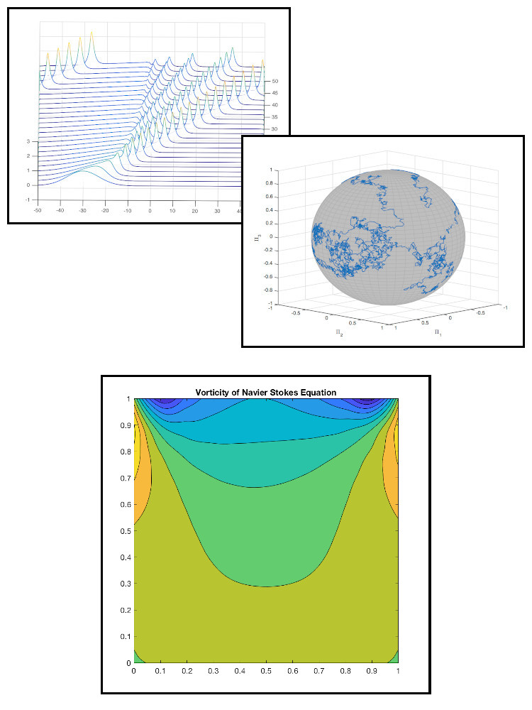
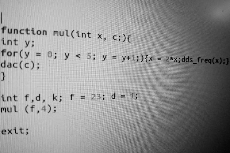
Bespoke Language
Project Description
Unlike most of the other project, this one does not deal much with applied mathematics. It concerns of designing, and implementing a bespoke programming language from scratch for a bespoke architecture. The goal of this programming language is to control laser pulse sequences for trapped ion quantum computer. The hardware included non-commercial and non-standard architecture, so a completely new compiler was required. Furthermore, the hardware lacked an arithmetic logic unit, thus a virtual machine was implemented to compensate for the missing unit. The addition of the virtual machine allows the use of many mathematical function to be used in the programming language. The compiler and the virtual machine are implemented in C and the Flex + Bison are used for the code parser. The project is a closed source, so no code is posted on Github.
Sparse Grids
Project Description
As I am interested in numerical schemes, and as a part of exploring adaptive schemes for multisymplectic integrators, I delved into sparse grids. One of their primary use is in quadrature of high dimensional integrals. Applying the quadrature methods and techniques designed for low-dimensional integrals, one would run into the dreaded curse of dimensionality, where it is required the use of \(\mathcal{O}(N^d)\) nodal points to evaluate a d-dimensional integral using \(N\) grid point per dimension. One method to mitigate the effects of curse of dimensionality, is the sparse grid method, where the number of grid points needed is \(\mathcal{O}(N(\mathrm{log}(N))^{d-1})\). The main ingredient of the sparse grid method is the tensor product of one-dimensional hierarchical basis.
Sparse grids are not only used for approximating high-dimensional integrals, but it can be used to define adaptive quadrature methods for high-dimensional problems. In recent years, sparse grids have been applied to a number of problems from data mining to computational finance, where they are used for the valuation of multi-asset options.
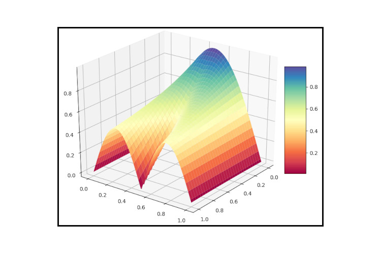
The following two figures show the use of adaptive sparse grids in the approximating the quadrature of the two-dimensional function
$$ f(x,y) = \frac{1}{|0.5 - x^2 -y^2| + 0.1} $$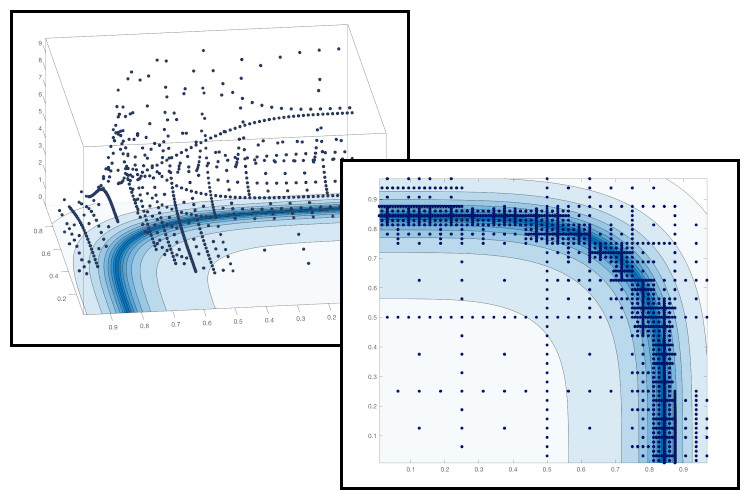
Motion Planning of Linear PDEs
Project Description
This project focuses on finding the optimal control for the heat equation implementing a finite approximation instead. Idea behind using an a discretised system is to allow us to apply the theory of optimal control for linear finite-dimensional systems to a partial differential equation. The control system is the same as in Laroche et al. paper "Motion Planning For the Heat Equation", however, here the approach is different than the approach they presented.
Here we show that the optimal control for a linear parabolic partial differential equation, the heat equation namely, can be obtained by using methods developed primarily for systems whose evolution is governed by a linear ordinary differential equation. In general optimal control of partial differential equations can be challenging, and one way to circumvent these challenges is to approximate the partial differential equation to a system of ordinary differential equation by using finite differencing.
Consider the 1D heat equation, which is a linear parabolic partial differential equation, $$ \begin{aligned} \begin{cases} &\partial_t \phi - \kappa \partial_{xx}\phi = 0, \quad (x,t) \in [0, 1] \times [0,T],\\ &\phi(0, t) = u(t),\\ &\partial_x \phi(1, t) = 0, \\ &\phi(x,0) = \phi_0(x), \quad \phi(x, T) = \phi_T(x), \end{cases} \end{aligned} $$ where \(\kappa > 0 \) is the diffusion rate. The optimal control problem deals with finding $u$ such that the heat equation is fulfilled and in the same time minimising the following cost functional $$ J(u) = \frac{1}{2}\int_0^T u^2 \, dt $$ Before discussing the approach we are using to solve this problem, we briefly summarise the fundamentals of control of linear finite-dimensional systems. Consider the linear control system given by $$ \dot{x}= A x + Bu(t), $$ where \(x \in \mathbb{R}^N\), \(A \in \mathbb{R}^{N\times N}\), \(B \in \mathbb{R}^{N\times M} \)and \(u \in \mathbb{R}^M\). The optimal control \(u\), that stears makes \(x\) follow a trajectory such that \(x(t_0) = x_0\) and \(x(t_1) = x_T\), is given by the expression $$ u(t) = -B^T \Phi(t_0,t)^T W_c^{-1}(t_0,t1) \left( x_0 - \Phi(t_0,t_1)x(t_0)\right), $$ where \(\Phi(s,t) = e^{\int_s^t A(\tau) d\tau)} \) is the state transition matrix for \(A\), and \(W_c\) is the controllability Grammian and it is defined by $$ W_c(t_0, t_1)= \int_{t_0}^{t_1} \Phi(\tau,t_1)BB^T \Phi^T(\tau,t_1) d\tau. $$
Using the finite differencing method to approximate the heat equation For a given linear system of equations $$ \begin{aligned} \mathbf{\dot{u}} &= A \mathbf{u} \end{aligned} $$ it can be driven from the state \(\phi(t_0,x) \) at \(t_0\) to \(u(t_1, x)\) at \(t_1\) and that is by adding the term \(\theta(t)\). Hence the system of linear equations would become $$ \dot{\Phi }(t) = A \Phi(t) + Bu(t), $$ where \(\Phi \in \mathbb{R}^N\), such that \(\Phi_i(t) = \phi(x_i, t)\), and the vector \(B\) is used to choose which state should the controller control directly. From the setting of the problem $$ \begin{aligned} B = \begin{cases} B_i = 1 &, i = N \\ B_i = 0 &, \text{ otherwise} \\ \end{cases} \end{aligned} $$ Having discretised heat equation, the state transition matrix is given by $$ \Phi(s,t) = e^{(t-s) A}, $$ and the controllability Grammian \(W_c\) is given by $$ W_c(t_0, t_1)= \int_{t_0}^{t_1} e^{(t-\tau) A}BB^T e^{(t-\tau) A^T} d\tau. $$ Now we can evaluate the optimal control which yields $$ u(t) = -B^T \Phi(0,t)^TW_c(0, t)^{-1}( x_T - \Phi(0,t)x_0) $$
References:
[1] - B. Laroche, P. Martin, and P. Rouchon. "Motion planning for the heat equation." in International Journal of Robust and Nonlinear Control: IFAC‐Affiliated Journal 10.8 (2000): 629-643.
Smoothed Particle Hydrodynamics
Project Description
Smoothed particle hydrodynamics is a numerical method for solving hydrodynamic equations and it relies on Lagrangian viewpoint of fluids. It works by dividing the fluid into particles and each particle contains information about the fluid, such as velocity and density. These particles interact with each other and their interaction mirrors the dynamics of the fluid. The implementation was done in C++, and the main aim was to extend Smoothed Particle Hydrodynamics to simulate stochastic fluid partial differential equations.
This project's repository can be found here
Lattice Boltzmann Method
Project Description
Lattice Boltzmann Method is a computational fluid dynamics method for simulating incompressible fluids. My introduction to the method came during a course on computational fluid dynamics. I was fascinated by the method and at the same time I was looking for a fast numerical scheme to model water flow around the surface of a sail boat. This project's aim was solely to hone my C++ programming skills and study different boat designs.
Lattice Boltzmann Method's roots lie in kinetic gas theory, where the gas particles interact by collision. The interaction of particles amongst each other is not computed explicitly, however the statistical distribution is and it evolves according to the Boltzmann equation.
$$ \partial_t f + v \cdot \nabla f = \Omega, $$ where \(f(x,v,t)\) is the probability density of finding the particle at position \(x\) with a velocity \(v\). As the name of the numerical method suggests, the Boltzmann equation is solved on a discrete grid.Unlike normal grid methods, the grid used here discretises the direction of velocities \(c_i\). The model used in this project is the so-called \(D3Q19\) model, where each cell in a three dimensional space, has 19 possible direction. A probability density value, \(f_i\), is assigned to each velocity \(c_i\). The fluid particles are fixed in space, instead, their probability densities are exchanged. The Boltzmann equation on a discrete grid is $$ f_i(x + c_i \Delta t, t + \Delta t) = f_i(x,t) + \frac{1}{\tau}\left( f_i^{eq}(x,t) - f_i(x,t) \right) $$
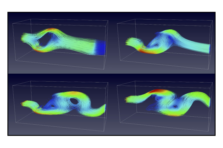
Using the Chapman–Enskog expansion, the solution of the lattice Boltzmann method approximates the solution of the incompressible Navier-Stokes equation. Furthermore, the scheme does not require solving algebraic equations, just substitutions, which makes it quicker than the standard finite volume method used for solving the Navier-Stokes equation.
One of the reasons why lattice Boltzmann method is attractive is due to ease of implementation and also it can be parallelised and it was an opportunity for me to practice implementing MPI codes. The figures show the streamlines of the numerical flow, with an obstacle in the channel, at three different times, and it is evident that the flow is experiencing von Kármán vortex street phenomenon.